
In this example, I will be using the open source solver, simpleFOAM to solve the two-dimensional turbulent flow over a backward-facing step with a Reynolds number of Re = 5100. This Reynolds number is based on the step height, h = 0.1m as shown in Figure 1. I will be using the incoming velocity 


Figure 1: Geometry for turbulent flow over a backward-facing step.
Here are the sections of this post:
- Case-setup and Boundary Conditions
- Grid convergence study
- Results and Validation
- Conclusion
- Some Useful References
Download the case file here: SA-CaseFile
Assumptions
- Incompressible flow
- Turbulent flow
- Newtonian flow
- 2-Dimensional flow
- Negligible gravitational effects
- Sea level conditions
- RANS turbulence modelling without wall functions
Case Setup and Boundary Conditions
The boundary specifications are; an incoming turbulent intensity of 10% which corresponds to a turbulent kinetic energy of 
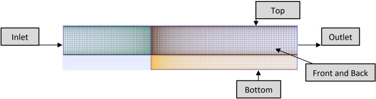
Figure 2: quadrilateral mesh.
k-epsilon Boundary Conditions Setup

Calculations of  and
and 
The turbulent kinetic energy,whereis the mean velocity inlet. For turbulent intensity of
, the turbulent kinetic energy is
whereis the turbulent viscosity ratio. For internal flows
,
. Therefore,
.

SA Boundary Conditions Setup
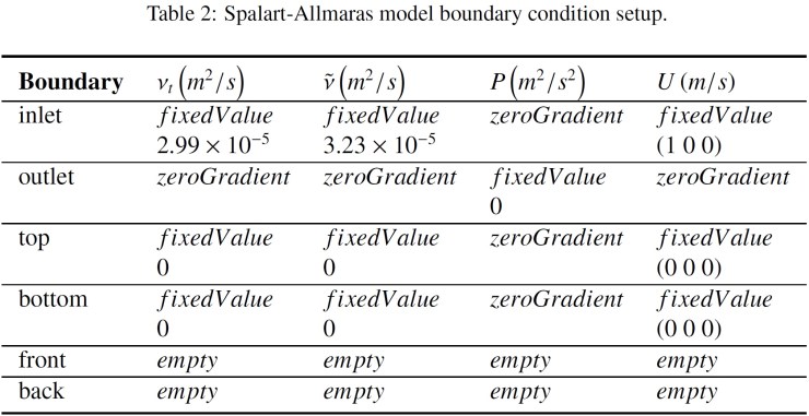
Calculations of  and
and 
The turbulent eddy viscosity is computed from:
where
where
is a viscous damping function and $latex C_{\nu 1}$ is a constant equal to 7.1.
where
and


k-omegaSST Boundary Conditions Setup

Calculations of and 
The turbulent kinetic energy,wherewhere
Grid Convergence Study
Three grids were made with number of nodes 7063, 29000, and 116248 respectively. According to NASA calculator for Re =5100 and ref. length 0.1, mesh spacing for the fine mesh should be 0.0002529. Mesh spacing for both the coarse mesh and medium were 0.0007529 and 0.0005529 respectively. Bases on the three grids, a grid convergence study was performed for each turbulent model to see how the results would vary. The three meshes used for


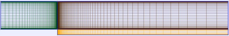

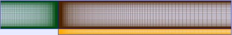
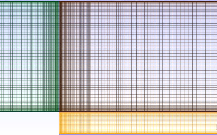

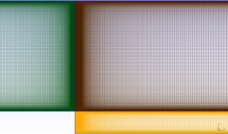
Figure 3: Shows coarse, medium, and fine mesh used for
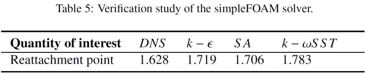
Results and Verification


Figure 4: Shows the pressure and velocity distributions for each turbulent models used for the simulation.
From extremely accurate direct numerical simulations (DNS), it has been determined that the reattachment of the separated boundary layer occurs on the bottom wall at
Conclusion
simpleFOAM has been verified for a classic example of an internal flow of a backward-facing step using three turbulent models in order to compare the results and how they affect the quantity of interests i.e. reattachment point. It has shown a great convergence study for the reattachment point. Boundary conditions for Spalat-Allmaras have been set up properly to resolve the boundary layer as well as 

Hi my friend. Congratulations for this work.
In the “Calculations for k and omega” you presented the same development in the “Calculations for k and epsilon”. What did you do to calculate de omega at the inlet?
Thank you very much!
LikeLike