Laminar Flow Over A Circular Cylinder

A common practice to verify and validate the OpenFOAM solver is the laminar two-dimensional flow around a cylinder. In this example, I will solve this problem using the simpleFOAM solver, which a steady state for incompressible Newtonian fluids. To begin, consider the two-dimensional flow around a cylinder with radius $R_{cyl}= 0.5m$ . The far-field boundary at a radius of $R_{max}= 10m$ .

problem2

Figure 1: Problem Description.

Using the given incoming velocity $V= 1m/s$ , density $\rho= 1kg/m^3$ , as well as the dynamic viscosity of $\mu= 0.025N.s/m^2$ , one can calculate the Reynolds as follows;

$Re= \dfrac{\rho U_{\infty} 2R_{cyl}}{\mu}=40$

Here are the sections of this post:

Assumptions
Case-setup and grid Generations
Drag Calculations
Grid convergence study
Validation
Conclusion

Download the case file here: Laminar-Flow-over-a-cylinder

Assumptions

Incompressible flow
Laminar flow
Newtonian flow
2-Dimensional flow
Negligible gravitational effects
Sea level conditions

Case setup and Grid Generations

Again, the purpose of this test is to verify and validate simpleFoam’s ability to predict the flow structure against the experimental result. The present calculation was confined to the low-Reynolds-number regime $Re=40$ , which encompasses steady symmetrical separated.

The no-slip wall condition is applied to the cylinder wall. Uniform free stream conditions are applied at the inlet and outlet boundaries.

Figure 2: Quadrilateral mesh.

Drag Calculations

The drag force coefficient $C_{d}$ of the cylinder is determined using the force function in OpenFOAM. The force function calculates the forces and moments by integrating the pressure and skin-friction forces over a given list of patches, and the resistance from porous zones. Then the drag coefficient $C_{d}$ is calculated by summing both forces on specified patches and normalize it to the dynamic free-stream pressure as in the following two equations;

$F = F_{pressure}+F_{Viscous}=\oint \left( p-p_{ref}\right)dA + \oint \mu\dfrac{du}{d\overrightarrow {n}} dA$

$\vec{F_{d}} = \vec{F}_{pressure}+\vec{F}_{viscous}=\sum_{i} \rho_{i} \vec{s}_{f,i} \left(p_i - p_{ref}\right)+\sum_{i} \vec{s}_{f,i} \cdot \left(\mu R_{\mathrm{dev}} \right)$

$C_{d} = \dfrac{F_{d}}{0.5\rho U_{\infty}^2 A_{cyl}}$

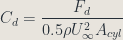
where $p_{i}$ is the local pressure at the wall surface, $p_{ref}$ is the reference pressure used to reduce round-off error during the computation of pressure force, $\mu$ denotes the dynamic viscosity of air, $R_{\mathrm{dev}}$ represents the velocity gradient at the wall surface. Furthermore, $U_{\infty}$ is the incoming velocity and $A_{cyl}$ is the area of the cylinder section.

Grid convergence study

All grids were generated using the open source software Gmsh. Three different resolutions figure (3) were made of the same family of meshing with spacing 0.05, 0.01, and 0.008 respectively. Based on the selected grids, simpleFOAM was run on each grid to obtain the value in which I decided to make my study. In this case, I chose the drag coefficient for each grid resolution table 1 and figure 4.

This slideshow requires JavaScript.

Figure 3: Shows coarse, medium, and fine mesh grids.

CdvsNCyl

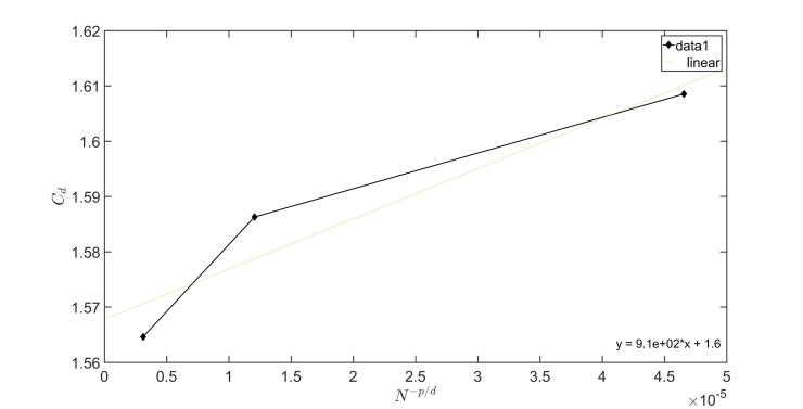
Figure 4: Grid convergence for the flow over a cylinder.

Since the simpleFOAM is a second order accurate, hence, P in table 1 is the effective order of convergence, and d is the number of spatial dimensions. Therefore, $P=2$ and $d=2$ . Hence, performing a Richardson extrapolation, and calculating the grid convergence index to ensure that you are in the asymptotic range of convergence. This can also be noted in table 1.

CGS

It should be noted from table 1 the pressure force is the dominant part i.e. pressure force = 0.51 in compared to viscous force=0.27. This indicates that most of the drag comes from the pressure force since pressure force comes from the eddying motions that are set up in the fluid by the passage of the body. While viscous force is important for attached flows (that is, there is no separation), and it is related to the surface area exposed to the flow, pressure force is important for separated flows, and it is related to the cross-sectional area of the body.

Results

Figure (5) shows one of the histories of convergence obtained during the simulations.

History of Convergenve

Figure 5: Shows an example of the convergence history for the flow over a cylinder.

Drag Coefficent

Figure 6: Shows the drag coefficient distributions vs. the number of iterations.

Cp dist. Coarse grid

Cp dist. Medium grid

Cp dist. Fine grid

V dist. Coarse grid

V dist. Medium grid

V dist. Fine grid

Figure 7: Shows the pressure and velocity distributions respectively for the three grids.

Validation

What is the predicted drag coefficient $C_{d}$ at this Reynolds number? Well, from experiments at this Reynolds number the approximated drag coefficient is approximately 1.65. From table 1, simpleFOAM predicted $C_{d}=1.602$ .

Conclusion

simpleFOAM has been validated for a classic example of external flows around a cylinder. The experimental data of the drag coefficient for Re=40 fairly agree well with the CFD data.

Some Useful References

Coutanceau, M. and Defaye, J.R., Circular Cylinder Wake Configurations – A Flow Visualization Survey, Mech. Rev., 44(6), June 1991.
http://www.calpoly.edu/~kshollen/ME554/Labs/validation_example.pdf.

Assumptions

Case setup and Grid Generations

Drag Calculations

Grid convergence study

Results

Validation

Conclusion

Some Useful References

Share this:

Like this:

Related

Leave a Reply Cancel reply