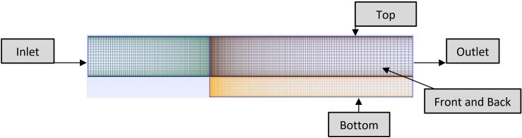
In this example, I will be using the open source solver, simpleFOAM to solve the two-dimensional turbulent flow over a backward-facing step with a Reynolds number of Re = 5100. This Reynolds number is based on the step height, h = 0.1m as shown in Figure 1. I will be using the incoming velocity , , and yielding for the dynamic viscosity. I will be utilizing three different turbulent models Spalart-Alamars, , and SST with the aim to test each model’s accuracy against other numerical data. From extremely accurate direct numerical simulations (DNS), it has been determined that the reattachment of the separated boundary layer occurs on the bottom wall at .
Figure 1: Geometry for turbulent flow over a backward-facing step.
Case Setup and Boundary Conditions
The boundary specifications are; an incoming turbulent intensity of 10% which corresponds to a turbulent kinetic energy of at the inlet. The outlet boundary is defined as an outflow condition while the no-slip condition is invoked for the rest of the computational walls. Show convergence histories, pressure contours for the entire flow region, and plot velocity vectors or pathlines. Discuss any observed flow characteristics. Use grids of varying densities to determine the sensitivity of the mesh to the reattachment point of the recirculation zone. Perform a grid convergence study using the reattachment location as the target quantity. Employ at least two different turbulence models.
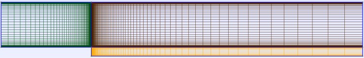
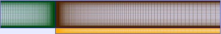
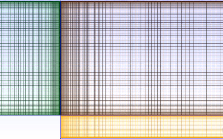
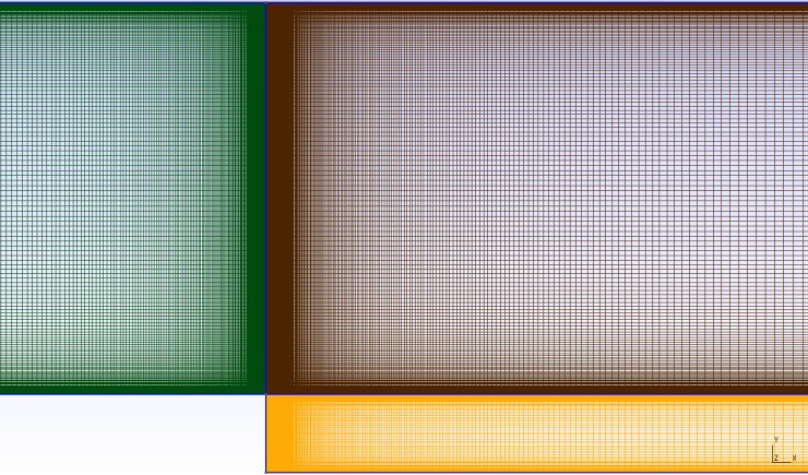
Figure 3: shows coarse, medium, and fine mesh for the same family of grids.
Results
Verification
From extremely accurate direct numerical simulations (DNS), it has been determined that the reattachment of the separated boundary layer occurs on the bottom wall at (note the origin of the coordinate system)