Flow Over A Flat Plate

An excellent test case to familiarize yourself with some of the turbulence models available in OpenFOAM is a 2D flat plate with zero pressure gradient. I will solve this problem using the solver simpleFOAM, which is a steady state solver for incomprehensible Newtonian fluids, utilizing the k- $\epsilon$ as well as Spalart Allmaras models. For the k- $\epsilon$ , I will be focusing on the use of wall function as well as finding a suitable y+ for the solution accuracy. Then I will verify k- $\epsilon$ results with NASA code for the skin friction coefficient. Finally for $u^+$ vs $y^+$ using Spalart Allmaras model with no wall function.

Here are the sections of this post:

Assumptions
Quick Overview: k- $\epsilon$ and SA Boundary Conditions
Case set-up and mesh and Boundary Conditions
Verification and Grid Convergence Study
Conclusions
Useful Resources

Download the case files here: Case-Files

Assumptions

Incompressible flow
Turbulent flow
Newtonian flow
2-Dimensional flow
Negligible gravitational effects
Sea level conditions
RANS turbulence modelling without wall functions

Quick Overview: k-epsilon Boundary Conditions

In this section, I will describe the boundary set-up for k- $\epsilon$ where wall functions are implemented see the figure 1. This requires that the y+ along the wall is greater than 30 see figure 1. For the k- $\epsilon$ turbulence model the boundary conditions are as follows:

LawofWall

Figure 1: Turbulence near the wall.

At the wall:

– specific dissipation rate
- BC type: epsilonWallFunction
- BC value: 0

k – turbulent kinetic energy
- BC type: kqWallFunction
- BC value: 0
nut – turbulent viscosity
- BC type: nutkWallFunction
- BC value: 0

See the following link

In the free-stream:

– specific dissipation rate
- BC type: fixedValue
- BC value: $1.04 \times 10^-4$

k – turbulent kinetic energy
- BC type: fixedValue
- BC value: $2.4 \times 10^-3$

nut – turbulent viscosity
- BC type: calculated
- BC value: 0 (this is just an initial value)

Calculations of $k$ and $\epsilon$

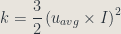
The turbulent kinetic energy, $k$ , and turbulent dissipation rate, $\epsilon$ , were calculated as:

$k=\dfrac{3}{2}\left( u_{avg}\times I\right)^{2}$

For external flows the value of turbulent intensity at the freestream can be as low as 0.05% depending on the flow characteristics. A good estimate of the turbulence intensity at the freestream boundary from experimentally measured data is approximately $I=0.058 \%$ . This leads to $k=2.4 \times 10^-3m^2/s^2$ . The turbulent dissipation rate, $\epsilon$ , is calculated as:

$\epsilon=C_{\mu}^{3/4}\dfrac{k^{3/2}}{l}$

where $u_{avg}$ is the mean velocity inlet, $l$ is length scale a $C_{\mu}$ is an empirical constant equal to 0.09. Length scale depends on the length of the wind tunnel and is calculated through the following formula:

$l=0.7\times L$

where, $L$ is the length of the flat plate. Thereby, this approximation or estimation to the turbulent dissipation rate, $\epsilon$ of $1.04 \times 10^-4$

Quick Overview: SA Boundary Conditions

At the wall:

– specific dissipation rate
- BC type: fixedValue
- BC value: 0

nut – turbulent eddy viscosity
- BC type: fixedValue
- BC value: 0

In the free-stream:

– turbulent viscosity
- BC type: fixedValue
- BC value: $2.92 \times 10^-6$

nut – turbulent eddy viscosity
- BC type: calculated
- BC value: 0 (this is just an initial value)

Calculations of $\nu_{t}$ and $\tilde{\nu}$

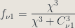
The turbulent eddy viscosity is computed from:

$\nu_{t}=f_{\nu1} \tilde{\nu}$

where

$f_{\nu1}=\dfrac{\chi^{3}}{\chi^{3}+C_{\nu1}^{3}}$

where $f_{\nu1}$ is a viscous damping function and $latex C_{\nu1}$ is a constant equal to 7.1.

$\chi=\frac{\tilde{\nu}}{\nu}$

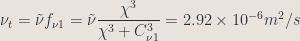
where $\chi=\beta$ and $\beta$ is the turbulent viscosity ratio, which is simply the ratio of turbulent to laminar (molecular) viscosity. For external flows, the freestream turbulent viscosity will be on the order of laminar viscosity so small, so values of β are appropriate, say $\beta= 1-10$ .

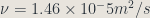
Furthermore, $\nu = \mu/\rho$ is the molecular kinematic viscosity, and \mu is the molecular dynamic viscosity. Therefore,

$\chi=\beta=3=\frac{\tilde{\nu}}{\nu} \Rightarrow \tilde{\nu}=3\nu=4.5\times 10^{-5} m^{2}/s$

$\nu_{t}=\tilde{\nu}f_{\nu1}=\tilde{\nu}\dfrac{\chi^{3}}{\chi^{3}+C_{\nu1}^{3}}=2.92\times 10^{-6} m^{2}/s$

Case set-up and mesh

Free-Stream Properties

For this case, I have followed a similar set up to the 2D flat plate case used on the NASA turbulence modelling resource website. This will help to gain more confidence be having data to verify the simpleFOAM solver. Since we are using simpleFOAM, I am going to set up the case file as suggested in this document, which uses a velocity (U) of 69.26 m/s see figure 2. The simulation properties that I used are :

FlatPlate

Figure 2: Schematic diagram of the problem.

$U_{\infty}=69.26 m/s$
$\nu=1.46 \times 10^-5 m^2/s$
$L=2 m$

These correspond to a Reynolds number at L=2m of 5 million.

Grid Generation

The grid was generated using Gmsh, which is also a very powerful open source software. High inflation was used in the boundary layer region new the wall in order to achieve the desired y+ value of less than 1 for the SA case.

FlatplateGrid — Figure 3: Shows the Grid and boundary conditions.

Boundary Conditions

For the incompressible simpleFOAM solver, the minimum boundary conditions required for a laminar flow simulation are p and U since for laminar flow, the fluid viscosity is large enough to damp out perturbations introduced to the flow, while for turbulent flows the inertial forces are much larger than the viscous forces. This implies that in order to to get the right physics, additional boundary conditions are required for the Navier-Stokes equations as the current problem is highly turbulent flow $Re=5million$ . simpleFOAM has numerous turbulence models implemented within OpenFOAM, and I will be using $k-\epsilon$ and SA in this post. For the $k-\epsilon$ model, we need to have a boundary condition on $k$ and $\epsilon$ as well. The boundary conditions I defined in the zero (0) folder can be found in the attached tutorial file.

Tip for fvSolution

If you find that the results you are getting are wrong, it could be that the residuals for the different properties are too high! Certain properties converge before others and therefore you need to ensure that they all converge to at least five orders of magnitude convergence!

Verification

For verification of the skin friction coefficient, I will be comparing the current simpleFOAM results using $\epsilon$ model for various $y^{+}$ values e.g. 20-300 against NASA data using CFL3D solver. The results are shown in figure 4. As can be noticed, there are certain $y^{+}$ values where the current solver predicts the NASA results reasonably well. Figure 5 illustrates the coefficient of skin friction using $y^{+}=40$ vs NASA solver. One can see from the figure that the coefficient of skin friction from our simulation matches the NASA data reasonably well.

Y+effect

Figure 4: Effect of $y^{+}$ on the solution accuracy using $k-\epsilon$ model.

FlatPlateV

Figure 5: Verification study of the coefficient of friction.

Next, let’s compare the $u^+$ vs $y^+$ profile to the universal profile for turbulent boundary layers. Recall that $u^+$ is the velocity normalized by the friction velocity $u_*$ , and $y^+$ is given by the following equation:

$y^+=\frac{u_*y}{\nu}$

The $u^+$ is vs $y^+$ is plotted here:

u+Vsy+

Figure 6: Verification study of the $u^+$ vs $y^+$ .

Figure 6: Verification study of the $u^+$ vs $y^+$ .

We can see from the figure that the current solution is in good agreement with CFL3D solver but with approximately 3% slight deviation at $y^{+} > 10^3$ . It should also be noted that the $y^+$ value of the first node is located around a y+ of approximately 0.5, the viscous sublayer matches very closely and the log law layer is not significantly off.

Conclusions

In this post, I simulated a zero pressure gradient flat plate at a Reynolds number of 5 million. I compared the results for $k-\epsilon$ model of the skin friction to the NASA turbulence modelling resource expected results and showed good agreement, and It was concluded that $y^+$ ranges from 30-50 was suitable enough to obtain accurate results. Then the $u^+$ vs $y^+$ profile was compared to the universal law of the wall and again the results were okay!

Category: Flow Over A Flat Plate