
Author: Tariq Khamlaj
CODES
Potential flow around a cylinder
The potential flow over a cylinder in the free stream is a common problem as it helps to examine numerical problem-solving techniques. The equation describing the potential flow over an object in two-dimensional flow reduces to the Laplace partial differential equation. Fortunately, the Laplace equation has a well-known solution and can be solved analytically. This provides a good benchmark to gauge the accuracy of the numerical approximation. The problem is the simplest form of Computational Fluid Dynamics, but the general algorithm forms the foundation for the higher fidelity models.
A cylinder was selected due to the availability of its analytical solution and for its simplicity. The numerical simulation was conducted by changing grid densities, calculating the order of convergence, and verifying with the exact solution
In this example, I implemented a second-order accurate potential flow solver for the flow around a cylinder using 


CURRICULUM VITAE
Flow Over A Flat Plate
An excellent test case to familiarize yourself with some of the turbulence models available in OpenFOAM is a 2D flat plate with zero pressure gradient. I will solve this problem using the solver simpleFOAM, which is a steady state solver for incomprehensible Newtonian fluids, utilizing the k-


Here are the sections of this post:
- Assumptions
- Quick Overview: k-
- Case set-up and mesh and Boundary Conditions
- Verification and Grid Convergence Study
- Conclusions
- Useful Resources
Download the case files here: Case-Files
Assumptions
- Incompressible flow
- Turbulent flow
- Newtonian flow
- 2-Dimensional flow
- Negligible gravitational effects
- Sea level conditions
- RANS turbulence modelling without wall functions
Quick Overview: k-epsilon Boundary Conditions
In this section, I will describe the boundary set-up for k-

Figure 1: Turbulence near the wall.
At the wall:
- BC type: epsilonWallFunction
- BC value: 0
- k – turbulent kinetic energy
- BC type: kqWallFunction
- BC value: 0
- nut – turbulent viscosity
- BC type: nutkWallFunction
- BC value: 0
In the free-stream:
- BC type: fixedValue
- BC value:

- k – turbulent kinetic energy
- BC type: fixedValue
- BC value:

- nut – turbulent viscosity
- BC type: calculated
- BC value: 0 (this is just an initial value)
Calculations of  and
and
The turbulent kinetic energy,For external flows the value of turbulent intensity at the freestream can be as low as 0.05% depending on the flow characteristics. A good estimate of the turbulence intensity at the freestream boundary from experimentally measured data is approximately. This leads to
. The turbulent dissipation rate,
whereis the mean velocity inlet,
is length scale a
is an empirical constant equal to 0.09. Length scale depends on the length of the wind tunnel and is calculated through the following formula:
where,is the length of the flat plate. Thereby, this approximation or estimation to the turbulent dissipation rate,


Quick Overview: SA Boundary Conditions
At the wall:
– specific dissipation rate
- BC type: fixedValue
- BC value: 0
- nut – turbulent eddy viscosity
- BC type: fixedValue
- BC value: 0
In the free-stream:
- BC type: fixedValue
- BC value:

- nut – turbulent eddy viscosity
- BC type: calculated
- BC value: 0 (this is just an initial value)
Calculations of  and
and
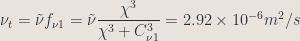
The turbulent eddy viscosity is computed from:
where
where
is a viscous damping function and $latex C_{\nu1}$ is a constant equal to 7.1.
where
and
is the turbulent viscosity ratio, which is simply the ratio of turbulent to laminar (molecular) viscosity. For external flows, the freestream turbulent viscosity will be on the order of laminar viscosity so small, so values of β are appropriate, say
.
Furthermore,
is the molecular kinematic viscosity, and \mu is the molecular dynamic viscosity. Therefore,


Case set-up and mesh
Free-Stream Properties
For this case, I have followed a similar set up to the 2D flat plate case used on the NASA turbulence modelling resource website. This will help to gain more confidence be having data to verify the simpleFOAM solver. Since we are using simpleFOAM, I am going to set up the case file as suggested in this document, which uses a velocity (U) of 69.26 m/s see figure 2. The simulation properties that I used are :

Figure 2: Schematic diagram of the problem.


These correspond to a Reynolds number at L=2m of 5 million.
Grid Generation
The grid was generated using Gmsh, which is also a very powerful open source software. High inflation was used in the boundary layer region new the wall in order to achieve the desired y+ value of less than 1 for the SA case.

Figure 3: Shows the Grid and boundary conditions.
Boundary Conditions
For the incompressible simpleFOAM solver, the minimum boundary conditions required for a laminar flow simulation are p and U since for laminar flow, the fluid viscosity is large enough to damp out perturbations introduced to the flow, while for turbulent flows the inertial forces are much larger than the viscous forces. This implies that in order to to get the right physics, additional boundary conditions are required for the Navier-Stokes equations as the current problem is highly turbulent flow 

Tip for fvSolution
If you find that the results you are getting are wrong, it could be that the residuals for the different properties are too high! Certain properties converge before others and therefore you need to ensure that they all converge to at least five orders of magnitude convergence!
Verification
For verification of the skin friction coefficient, I will be comparing the current simpleFOAM results using 


Figure 4: Effect of

Next, let’s compare the 

The

vs .We can see from the figure that the current solution is in good agreement with CFL3D solver but with approximately 3% slight deviation at 
Conclusions
In this post, I simulated a zero pressure gradient flat plate at a Reynolds number of 5 million. I compared the results for
Some Useful References
Flow Over NACA0012 Airfoil
In this example, the analysis of the two-dimensional subsonic flow over a NACA 0012 airfoil at various angles of attack and operating at a Reynolds number and Mach number 

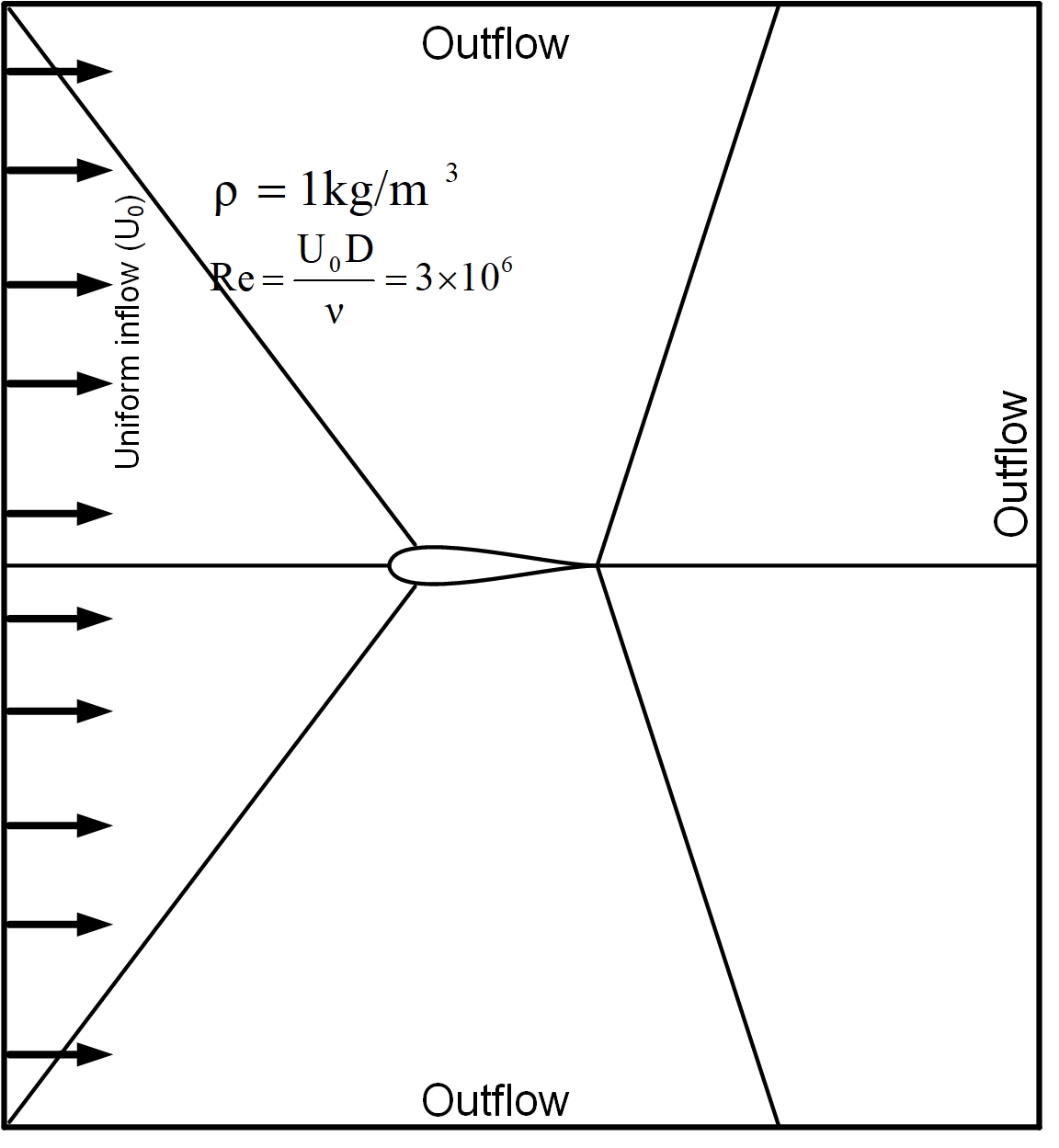
Figure 1: Geometry for turbulent flow over a backward-facing step.
Here are the sections of this post:
- Assumptions
- Case-setup and Boundary Conditions
- Grid convergence study
- Results and Verification
- Conclusion
- Some Useful References
- Future Work
Download the case file here.
Assumptions
- Incompressible flow
- Turbulent flow
- Newtonian flow
- 2-Dimensional flow
- Negligible gravitational effects
- Sea level conditions
- RANS turbulence modeling without wall functions
Case-setup and Boundary Conditions
The flow over NACA 0012 airfoil which is used in wind turbine blade is investigated using OpenFOAM, the steady incompressible solver simpleFoam with the SA model. Pressure and velocity coupling for the Navier-Stokes equation is solved by the SIMPLE algorithm. The convective term is discrete with the upwind scheme. A central scheme is used to discrete diffusion term and gradient term with a second order. Note that the boundary conditions for
Grid Convergence Study
Three types of grids are generated. For the fine grid, the computational domain was composed of 155608 cells emerged in a structured way, taking care of the refinement of the grid near the airfoil in order to enclose the boundary layer approach. Therefore, sets of y+ less than 1 in order to simulate sub-layer flow in the boundary layer are considered. Calculations were done for constant air velocity altering only the angle of attack for every turbulence model tested. Figure 2 shows a close-up view of the grid system provided for this case.

NACA 0012 airfoil grid

Fine grid

Medium grid

Coarse grid
Figure 2: Coarse, medium and fine grids used for the simulations.
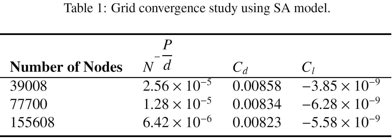
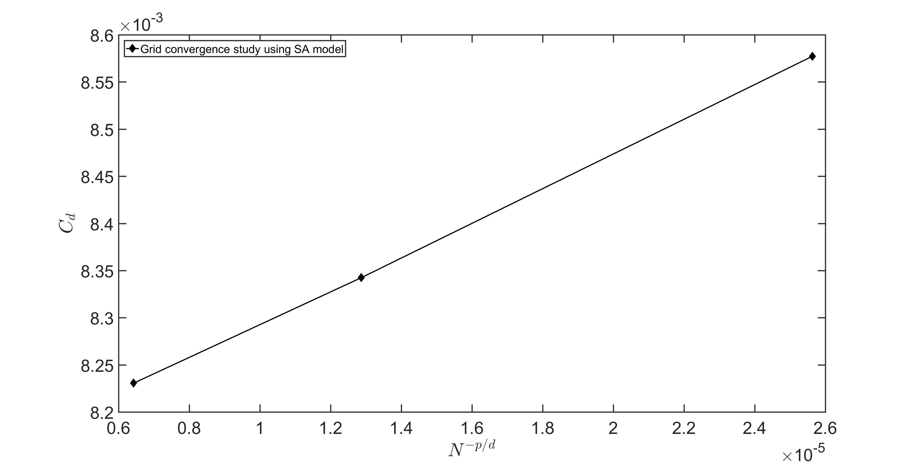
Figure 3: Grid convergence study for the drag coefficient vs. the number of nodes.
Results
Figure 4 illustrates the pressure and velocity distributions over NACA 0012 at zero angle of attack. As expected, the flow is fully symmetric.

Velocity distribution

Pressure distribution
As in the current case, a RAS model has been implemented, it is necessary to guarantee that the first node of the mesh falls within the viscous sublayer region. It is to ensure that 
Verification Study
Data for the lift and drag characteristics of the NACA 0012 airfoil were collected utilizing different CFD solvers. This airfoil was chosen because it has been used in many constructions. Typical examples of such use of the airfoil are the B-17 Flying Fortress and Cessna 152, the helicopter Sikorsky S-61 SH-3 Sea King as well as horizontal and vertical axis wind turbines.
The numerical values of lift and drag are given in Table 2, where I have adjoined data from CFL3D to data from the TMR website. Figures 5, 6, and 7 show pressure coefficient Cp over the airfoil surface of the airfoil for the three angles of attacks. The current results using OpenFOAM and CFL3D results are very close to one another.


Figure 5: Pressure coefficient, NACA0012, SA model OpenFOAM vs CFL3D.

Figure 6: Pressure coefficient, NACA0012, SA model OpenFOAM vs CFL3D.

Figure 7: Pressure coefficient, NACA0012, SA model OpenFOAM vs CFL3D.
The lift and drag coefficients are in very good agreement with other CFD solver results.
Conclusion
In this example, I showed the behavior of the 4-digit symmetric airfoil NACA 0012 at various angles of attack using the SA model. The predicted lift and drag coefficients were in good agreement with other CFD solver.
Some Useful References
- Eleni, Douvi C., Tsavalos I. Athanasios, and Margaris P. Dionissios. “Evaluation of the turbulence models for the simulation of the flow over a National Advisory Committee for Aeronautics (NACA) 0012 airfoil.” Journal of Mechanical Engineering Research 4.3 (2012): 100-111.
- Ahmed, Tousif, et al. “Computational study of flow around a NACA 0012 wing flapped at different flap angles with varying mach numbers.” Global Journal of Research In Engineering(2014).
- https://turbmodels.larc.nasa.gov/NAS_Technical_Report_NAS-2016-01.pdf
- Anderson Jr, John David. Fundamentals of aerodynamics. Tata McGraw-Hill Education, 2010.
- Excel datasheet for the pressure coefficient distribution.
Future Work
- I will be considering
SST model for future verification.
- I will be using the same mesh strategy on a vertical axis wind turbine to optimize both the pitch angle as well as the airfoil geometry.
