is the dimensionless wall distance for a wall-bounded flow. It can be expressed as:
where is the friction velocity , y is the distance to the nearest wall and is the kinematic viscosity of the fluid. is commonly used in boundary layer theory and in defining the law of the wall.
plays a relevant role in the treatment of the boundary layer. The subdivision of the near-wall region in a turbulent boundary layer can be summarized as follows:
: viscous sublayer region (velocity prole is assumed to be laminar and viscous stress dominates the wall shear).
: buffer region (both viscous and turbulent shear dominate)
: fully turbulent portion or log-law region (turbulent shear predominates)
Figure 1: Turbulence near the wall.
Figure 2: Law of the wall, horizontal velocity near the wall with mixing length model.
From figure 1, to use a wall function approach for a particular turbulence model with confidence, it is necessary to ensure that the values are within a certain range see Flow Over A Flat Plate example for the wall function use.
OpenFOAM presents a utility to calculate and report for all the wall patches. Note that as it depends on the local Reynolds number, it can only be obtained in the post-processing. Consequently, only approximate values can be estimated when meshing. When a RAS turbulence model is used, the instruction (written in the terminal) to obtain y+ is:
yPlusRAS
Notes:
In addition to the concern about having a mesh with y+ values that are too large, it is necessary to be aware that if the y+ is too low then the first calculation point will be placed in the viscous sublayer region and the wall function will also be outside its validity see Flow Over A Flat Plate example for the wall function use.
If an attached flow is modeled, then generally a wall function approach can be used. If flow separation is expected and the accurate prediction of the separation point will have an impact on the results then it would be advisable to resolve the boundary layer with a finer mesh.
Analysis and Optimization Study of Ducted Wind Turbines
Tariq Khamlaj & Markus Rumpfkeil
Abstract: Wind-lens turbines offer the potential for better energy efficiency and better suitability for urban and suburban environments compared to unshrouded or bare wind turbines. Wind-lenses, which are typically comprised of a diffuser shroud equipped with a flange, can enhance the wind velocity at the rotor plane due to the generation of a lower back pressure. In this article, the wind-lens efficiency is increased by designing the shroud and turbine shape as well as flange height through an optimization process that seeks to maximize the power while minimizing drag and thrust forces. The employed optimizer is a multi-objective genetic algorithm (MOGA). Bezier curves are used to define the chord and twist distribution of the turbine blades and a piecewise quadratic polynomial is utilized to define the shroud shape. The power, thrust, and drag coefficients are calculated by solving the Reynolds-averaged-Navier-Stokes (RANS) equations with the k-ε turbulence model for the flow within and around the diffuser augmented wind turbine using the open source code software OpenFOAM. To reduce the computational cost, the turbine rotor itself is modeled by incorporating blade element momentum model body forces into the RANS equations. Realistic rotor data for the sectional lift and drag coefficients for all angles of attacks are utilized via look-up tables. Grid convergence studies for verification and comparisons with experiments for validation are carried out to demonstrate that the adopted methodology is able to accurately predict the performance of a wind-lens prior to performing shape optimizations. It will be demonstrated that the resulting optimal designs yield significant improvements in the output power coefficient.
Theoretical Analysis of Shrouded Horizontal Axis Wind Turbines
Tariq Khamlaj & Markus Rumpfkeil
Abstract: Numerous analytical studies for power augmentation systems can be found in the literature with the goal to improve the performance of wind turbines by increasing the energy density of the air at the rotor. All methods to date are only concerned with the effects of a diffuser as the power augmentation, and this work extends the semi-empirical shrouded wind turbine model introduced first by Foreman to incorporate a converging-diverging nozzle into the system. The analysis is based on assumptions and approximations of the conservation laws to calculate optimal power coefficients and power extraction, as well as augmentation ratios. It is revealed that the power enhancement is proportional to the mass stream rise produced by the nozzle diffuser-augmented wind turbine (NDAWT). Such mass flow rise can only be accomplished through two essential principles: the increase in the area ratios and/or by reducing the negative back pressure at the exit. The thrust coefficient for optimal power production of a conventional bare wind turbine is known to be 8/9, whereas the theoretical analysis of the NDAWT predicts an ideal thrust coefficient either lower or higher than 8/9 depending on the back pressure coefficient at which the shrouded turbine operates. Computed performance expectations demonstrate a good agreement with numerical and experimental results, and it is demonstrated that much larger power coefficients than for traditional wind turbines are achievable. Lastly, the developed model is very well suited for the preliminary design of a shrouded wind turbine where typically many trade-off studies need to be conducted inexpensively.
Optimization Study of Shrouded Horizontal Axis Wind Turbine
Tariq Khamlaj & Markus Rumpfkeil
Abstract: There is a large interest in wind turbines which are suitable for urban and suburban environments in order to bring power production closer to the consumer to minimize transportation power losses. A prime candidate for these kinds of applications is a wind-lens. Wind-lenses, which consist of a diffuser shroud equipped with a brim, have the potential to increase the wind speed at the rotor due to the generation of a low back pressure region through vortex formation. The objective of this study is to improve the wind-lens efficiency by designing the duct and brim shape through an optimization process that maximizes the power while minimizing drag for a given turbine rotor shape. The optimization process is carried out by the DAKOTA software package developed by Sandia National Labs. The power and drag coefficients are calculated by employing the Reynolds-averaged-Navier-Stokes (RANS) equations to simulate the flow within and around a diffuser augmented wind turbine with a brim. The open source code OpenFOAM is used and in order to reduce the computational cost, the turbine rotor is represented via an axisymmetric CFD-integrated blade element momentum model (also known as actuator disk model). Realistic rotor data, such as local chord lengths and twist angles as well as the sectional airfoils’ lift and drag coefficients for all angles of attacks, are utilized in the blade element model. Grid convergence studies for verification and comparisons with experiments for validation are carried out to demonstrate that the adopted methodology is able to predict the performance of a wind-lens accurately prior to performing shape optimizations. It will be demonstrated that the optimum designs yield significant improvements in the output power coefficient.
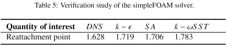
In this example, I will be using the open source solver, simpleFOAM to solve the two-dimensional turbulent flow over a backward-facing step with a Reynolds number of Re = 5100. This Reynolds number is based on the step height, h = 0.1m as shown in Figure 1. I will be using the incoming velocity , , and yielding for the dynamic viscosity. I will be utilizing three different turbulent models Spalart-Alamars, , and SST with the aim to test each model’s accuracy against other numerical data. From extremely accurate direct numerical simulations (DNS), it has been determined that the reattachment of the separated boundary layer occurs on the bottom wall at .
Figure 1: Geometry for turbulent flow over a backward-facing step.
The boundary specifications are; an incoming turbulent intensity of 10% which corresponds to a turbulent kinetic energy of at the inlet. The outlet boundary is defined as an outflow condition while the no-slip condition is invoked for the rest of the computational walls. Show convergence histories, pressure contours for the entire flow region, and plot velocity vectors or pathlines. Discuss any observed flow characteristics. Use grids of varying densities to determine the sensitivity of the mesh to the reattachment point of the recirculation zone. Perform a grid convergence study using the reattachment location as the target quantity. Employ at least two different turbulence models.
Figure 2: quadrilateral mesh.
k-epsilon Boundary Conditions Setup
Calculations of and
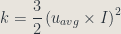
The turbulent kinetic energy, , and turbulent dissipation rate, , were calculated as:
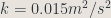
where is the mean velocity inlet. For turbulent intensity of , the turbulent kinetic energy is . The turbulent dissipation rate, , is calculated as:
where is the turbulent viscosity ratio. For internal flows may be scaled with the Reynolds numbers. In our case, for , . Therefore, .
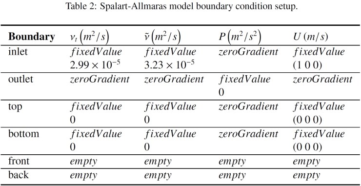
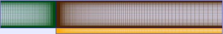
SA Boundary Conditions Setup
Calculations of and
The turbulent eddy viscosity is computed from:
where
where is a viscous damping function and $latex C_{\nu 1}$ is a constant equal to 7.1.
where and is the turbulent viscosity ratio, which is simply the ratio of turbulent to laminar (molecular) viscosity. For internal flows may be scaled with the Reynolds numbers. In our case, for , . Therefore,
k-omegaSST Boundary Conditions Setup
Calculations of and
The turbulent kinetic energy, , and specific dissipation rate, , were calculated as:
where is the mean velocity inlet. For turbulent intensity of , the turbulent kinetic energy is . The turbulent dissipation rate, , is calculated as:
where is the turbulent viscosity ratio. For internal flows may be scaled with the Reynolds numbers. In our case, for , . Therefore, .
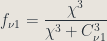
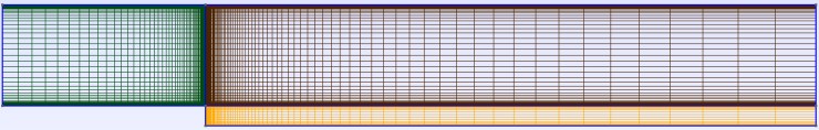
Grid Convergence Study
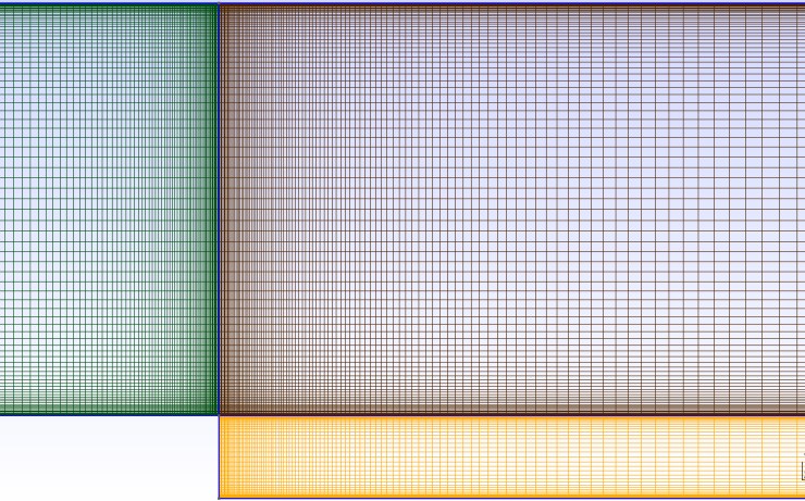
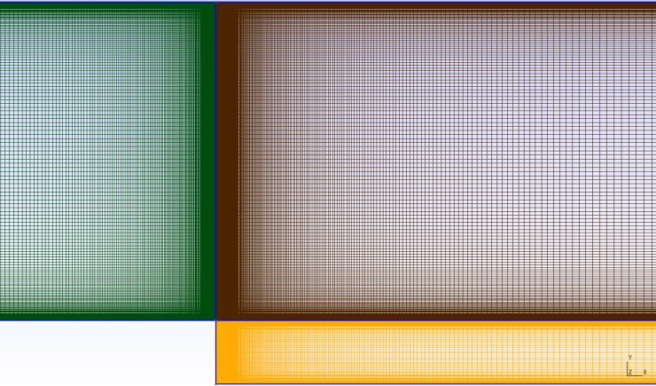
Three grids were made with number of nodes 7063, 29000, and 116248 respectively. According to NASA calculator for Re =5100 and ref. length 0.1, mesh spacing for the fine mesh should be 0.0002529. Mesh spacing for both the coarse mesh and medium were 0.0007529 and 0.0005529 respectively. Bases on the three grids, a grid convergence study was performed for each turbulent model to see how the results would vary. The three meshes used for SST model are shown in Figure (3). Table 4 provides the grid convergence study results for SST model.
Coarse gridCloser view of the coarse grid.Medium gridCloser view of the medium grid.Fine gridCloser view of the fine grid.
Figure 3: Shows coarse, medium, and fine mesh used for SST model.
Results and Verification
k-epsilon v dis.
k-omega v dis.
SA v dis.
SA p dis.
k-omega p dis.
k-epsilon p dis.
Figure 4: Shows the pressure and velocity distributions for each turbulent models used for the simulation.
From extremely accurate direct numerical simulations (DNS), it has been determined that the reattachment of the separated boundary layer occurs on the bottom wall at (note the origin of the coordinate system)
Conclusion
simpleFOAM has been verified for a classic example of an internal flow of a backward-facing step using three turbulent models in order to compare the results and how they affect the quantity of interests i.e. reattachment point. It has shown a great convergence study for the reattachment point. Boundary conditions for Spalat-Allmaras have been set up properly to resolve the boundary layer as well as with wall function (i.e. ) and SST without wall function. Furthermore, a comparison between DNS and simpleFOAM for the reattachment point show reasonable agreements.


: viscous sublayer region (velocity prole is assumed to be laminar and viscous stress dominates the wall shear).
: buffer region (both viscous and turbulent shear dominate)
: fully turbulent portion or log-law region (turbulent shear predominates)


 ,
,  , and
, and  yielding
  for the dynamic viscosity. I will be utilizing three different turbulent models Spalart-Alamars,
  , and
, and  SST with the aim to test each model’s accuracy against other numerical data. From extremely accurate direct numerical simulations (DNS), it has been determined that the reattachment of the separated boundary layer occurs on the bottom wall at
  .
.
 at the inlet. The outlet boundary is defined as an outflow condition while the no-slip condition is invoked for the rest of the computational walls. Show convergence histories, pressure contours for the entire flow region, and plot velocity vectors or pathlines. Discuss any observed flow characteristics. Use grids of varying densities to determine the sensitivity of the mesh to the reattachment point of the recirculation zone. Perform a grid convergence study using the reattachment location as the target quantity. Employ at least two different turbulence models.
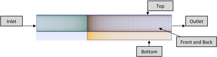

 and
and 
 is the mean velocity inlet. For turbulent intensity of
  ,
,
 is the turbulent viscosity ratio. For internal flows
  ,
,  . Therefore,
 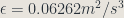 .
.
 and
and 

 is a viscous damping function and $latex C_{\nu 1}$ is a constant equal to 7.1.
 and
and 


 ) and
) and 